feeLLGood – NIST standard problem #4
The NIST has proposed a set of five standard micromagnetic problems that are useful for comparing micromagnetic simulation techniques. Among those, the standard problem #4 is the most widely used for validating implementations. This guide shows how this problem can be tackled with feeLLGood.
Problem definition
The sample is a thin slab of permalloy measuring 500 nm × 125 nm × 3 nm along x, y and z respectively. The magnetization is initially in a remanent s-state, which can be obtained “after applying and slowly reducing a saturating field along the [1,1,1] direction to zero”.
At t = 0, a magnetic field large enough to reverse the magnetization is instantly applied, and the system is left to evolve until it reaches its new equilibrium. The applied field can be either of:
- field 1: (−24.6, +4.3, 0) mT
- field 2: (−35.5, −6.3, 0) mT
In this guide, we will simulate only the response to the second field, which is the most sensitive to differences in solver implementations. The response to the first field can be simulated in exactly the same manner.
Meshing the sample
A simple way of creating the mesh is to use the “meshMaker” Python module, which is provided with feeLLGood. Specifically, the Cuboid function. We choose the nanometer as our unit, and we put the origin at the center of the sample. Then, the coordinates within the sample span the following ranges:
- x ∈ [−250, +250]
- y ∈ [−62.5, +62.5]
- z ∈ [−1.5, +1.5]
The following script, named “mksample.py”, will generate the mesh:
from feellgood.meshMaker import Cuboid

# Cuboid: 500 x 125 x 3 nm^3
corner_low = [-250, -62.5, -1.5]
corner_high = [250, 62.5, 1.5]

sample = Cuboid(corner_low, corner_high, 250, 63, 2)
sample.make("sample.msh", "volume", "surface")
Note that the last three parameters of the Cuboid function are the number of intervals (not nodes) into which each dimension is sliced. The slab is thus cut into 250×63×2 = 31,500 cuboids measuring 2×1.98×1.5 nm3. Their size long z may seem too small. However, for the accuracy of the finite element formulation, it is important to have more than one layer of elements in the sample thickness. Each cuboid is then split into six tetrahedra, for a total of 189,000 tetrahedra. The mesh will have 251×64×3 = 48,192 nodes. This is confirmed by running the script:
$ python3 mksample.py
Generated sample.msh: 48192 nodes, 189000 tetrahedra
Initial state
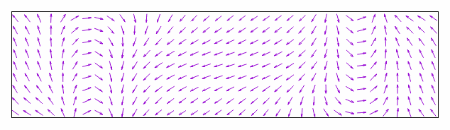
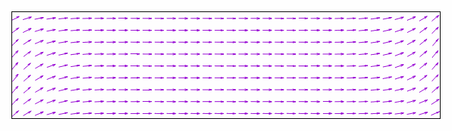
As per the problem statement, the initial state can be achieved by applying a large field along [1,1,1], and slowly decreasing it to zero. This, however, is a lengthy procedure. As we know what the remanent state looks like, we can reach it faster by initializing the sample in an ansatz (or analytical approximation) of the desired state, then letting it relax with no applied field. As an ansatz we choose:
m = m′/‖m′‖
m′ = (1, (x/250 nm)8, 0)
This has the magnetization aligned mostly along the +x direction, except near the ±x edges of the sample, where it deviates by 45° from this direction. This ansatz is depicted below:
Now we ask feeLLGood to relax this magnetic state, using the following settings file. The material parameters are taken from the original problem definition, save for the α damping constant, which is set to 1 in order to speed up the relaxation:
# Relax towards the S state.

outputs:
  directory: relax.d
  file_basename: relax
  evol_time_step: 5e-12
  final_time: 1e-7
  evol_header: true
  take_photo: 10
mesh:
  filename: sample.msh
  scaling_factor: 1e-9
  volume_regions:
    volume:
      Ae: 1.3e-11
      Js: 1.005309649696
      alpha_LLG: 1
  surface_regions:
    surface:
initial_magnetization: [1, (x/250e-9)**8, 0]
Bext: [0, 0, 0]
time_integration:
  max(du): 0.02
  min(dt): 1e-15
  max(dt): 5e-12
The relaxation can be monitored by plotting the evolution of the total energy, which feeLLGood writes to the file “relax.d/relax.evol”:
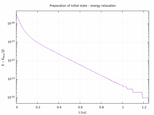
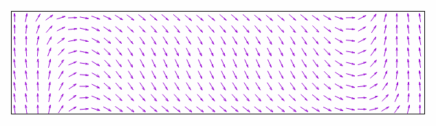
The staircase at the bottom right of the plot is due to the numerical resolution of the output file, which is limited to six significant decimal digits. After 1.2 ns, the system has practically reached its equilibrium. We nevertheless let it relax for longer, only to be sure it is completely relaxed. After about two hours of computation (7.765 ns of simulated time), feeLLGood was stopped with Ctrl-C. The remanent state can then be found in “relax.d/relax_at_exit.sol”:
In order to use this as the initial state for the next simulation, we rename the file “relaxed.sol”, and change the line showing the time of the snapshot, so that it reads:
## time: 0
Response to the applied field
For the actual simulation, we use this settings file:
# Apply "field 2": (-35.5, -6.3, 0) mT

outputs:
  directory: field2.d
  file_basename: field2
  evol_time_step: 5e-12
  final_time: 5e-9
  evol_header: true
  take_photo: 10
mesh:
  filename: sample.msh
  scaling_factor: 1e-9
  volume_regions:
    volume:
      Ae: 1.3e-11
      Js: 1.005309649696
      alpha_LLG: 0.02
  surface_regions:
    surface:
initial_magnetization: relaxed.sol
Bext: [-0.0355, -0.0063, 0]
time_integration:
  max(du): 0.02
  min(dt): 1e-15
  max(dt): 5e-12
This is almost identical to the previous one. Other than the file names and paths, the only relevant differences are:
- the damping constant is now α = 0.02, as per the problem definition
- the initial magnetization is given by our previous result
- the applied field is the problem's “field 2”
Here is the first nanosecond of the evolution of the average magnetization:
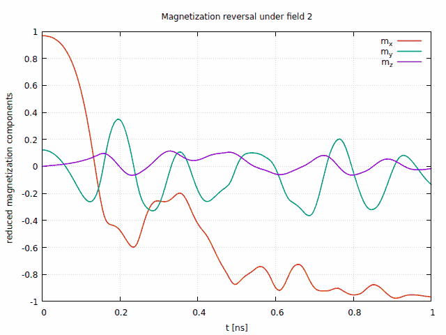
The my curve can be compared to the published results on the same problem. It is very similar to most of these results, and almost identical to the data submitted by José L. Martins and Tania Rocha.
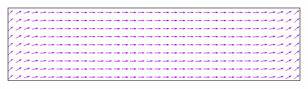
Let's look at the magnetic configuration in the middle of the reversal. The x component of the magnetization crosses zero at about 135.8 ps. Since we are recording a snapshot of the magnetization every 50 ps, the closest snapshot is at t = 150 ps: